
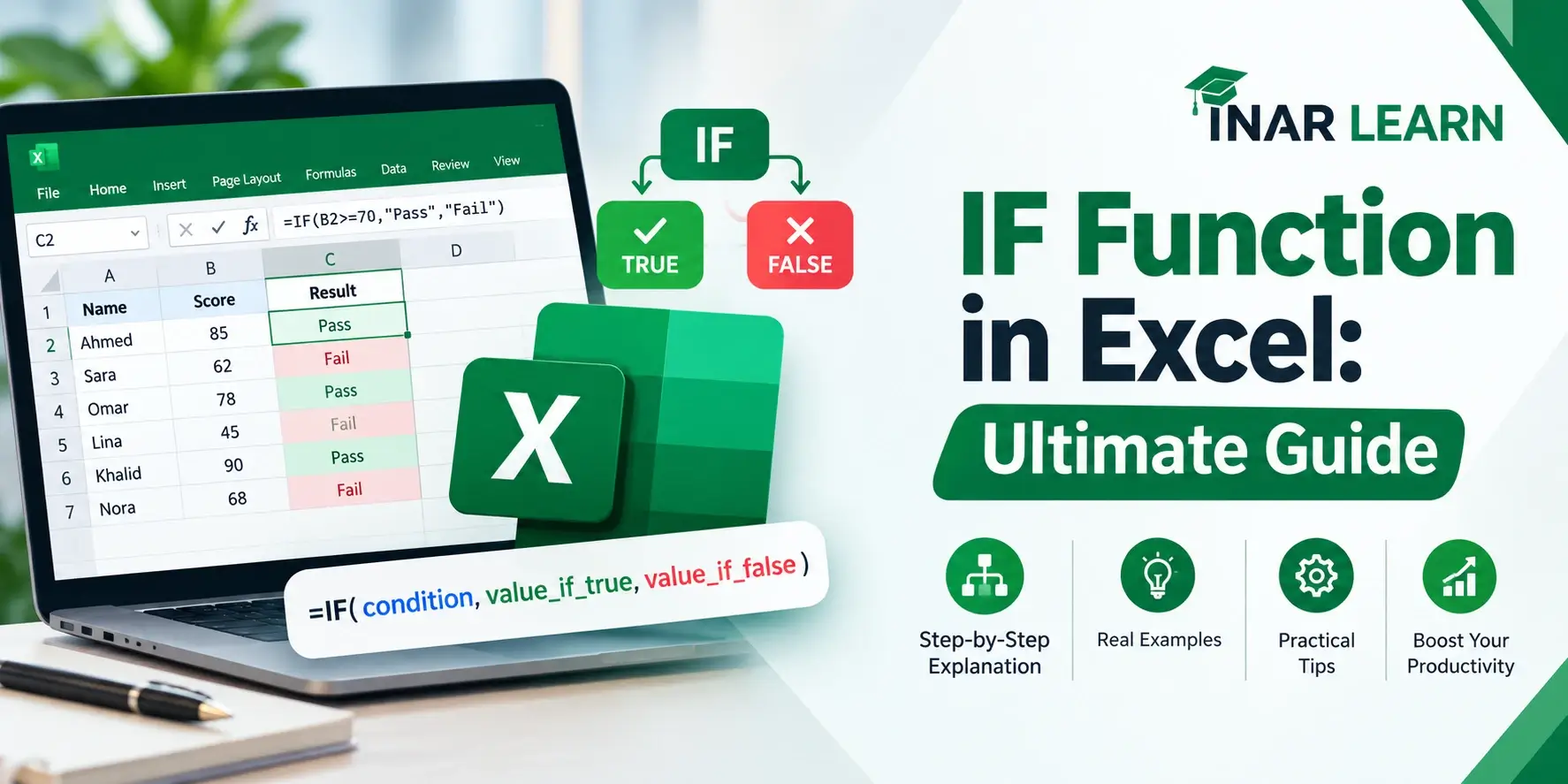
The IF function is where almost everyone starts with Excel formulas — and where almost everyone eventually writes a nine-level nested monster that nobody dares to edit. This guide walks through the whole thing with real spreadsheet examples you can type into a blank workbook today.
You will see the syntax broken down argument by argument, six comparison operators, a full worked payroll example, a grade tracker, a commission tier model, plus nested IF, IFS, AND/OR/NOT, text and wildcard tests, date logic, and the ways IF works together with lookups, data validation, and conditional formatting.
The IF function tests a condition and returns one value when the test is TRUE and another when it is FALSE, written as =IF(logical_test, value_if_true, [value_if_false]).
What Is the IF Function?
IF is Excel’s branching function. It evaluates a condition — the logical test — and then chooses between two outcomes. The condition must resolve to either TRUE or FALSE; there is no third state and no “maybe”.
That binary nature is the source of both its power and its limits. It is excellent for decisions with two outcomes: pass or fail, over budget or under, in stock or out. It becomes awkward the moment a decision has three or more possible outcomes, which is why nested IF exists and why IFS was added to Excel in 2019.
How IF evaluates a formula
Take the formula =IF(A2>=60, "Pass", "Fail"). Excel reads it in three steps:
- Evaluate the logical test. It computes
A2>=60and produces either TRUE or FALSE. Nothing else is looked at yet. - Pick the matching branch. If the test is TRUE, Excel reads the second argument. If FALSE, the third.
- Return that value. Only the chosen branch is evaluated — the other one is never computed, which matters if one branch contains an expensive lookup or a formula that could error.
Excel also has IFS, SWITCH, CHOOSE, and lookup functions like XLOOKUP. Each solves a slightly different shape of problem.
Syntax and Arguments
The full signature has three arguments, and only the last one is optional.
=IF(logical_test, value_if_true, [value_if_false])Walking through each argument
- logical_test — any expression that evaluates to TRUE or FALSE. Usually a comparison such as
A2>=60,B2="", orC2<>0. - value_if_true — what to return when the test is TRUE. Can be a number, text in double quotes, a cell reference, or another formula.
- value_if_false (optional) — what to return when the test is FALSE. If you omit it, Excel returns the logical value
FALSE.
| Argument | Required? | Notes |
|---|---|---|
logical_test | Required | Must resolve to TRUE or FALSE. Numbers count — 0 is FALSE, anything else is TRUE. |
value_if_true | Required | Text must be in double quotes: "Pass". |
value_if_false | Optional | If omitted, the cell shows the word FALSE when the test fails. |
Writing =IF(A2>=60,Pass,Fail) makes Excel look for defined names called Pass and Fail. It fails with #NAME?. Always wrap literal text in double quotes.
If you leave it out, a failed test returns the word FALSE in the cell. That is almost never what a report should show. Use "" for a blank-looking result, or 0 for a numeric one.
Comparison Operators
The logical test is built from comparison operators. These are the six you will use in almost every IF formula you ever write.
| Operator | Meaning | Example | TRUE when… |
|---|---|---|---|
= | Equal to | A2="Yes" | A2 contains the text Yes |
> | Greater than | A2>100 | A2 holds a number above 100 |
< | Less than | A2<0 | A2 holds a negative number |
>= | Greater or equal | A2>=60 | A2 is 60 or higher |
<= | Less or equal | A2<=100 | A2 is 100 or lower |
<> | Not equal to | A2<>"" | A2 is not empty |
Boundary values — where most bugs live
The single most common off-by-one bug in an IF formula is choosing > when you meant >=. The two differ only at the exact threshold, which is precisely the case that gets tested in reports.
| A Score | B >=60 | C >60 | |
|---|---|---|---|
| 2 | 59 | Fail | Fail |
| 3 | 60 | Pass | Fail |
| 4 | 61 | Pass | Pass |
>= and fails with >. Decide which behaviour you actually want before you write the formula.When a formula misbehaves, paste just the logical test into an empty cell — for example =A2>=60 on its own. It returns TRUE or FALSE, which tells you whether the problem is the test or the branches.
Real-World Examples
These are the patterns that come up over and over in actual workbooks. Each one includes a spreadsheet mockup showing exactly what the data looks like and the formula that goes in each cell.
Example 1 — Payroll: overtime pay calculation
Pay the standard rate up to 40 hours, and 1.5× the rate for any hours beyond 40.
| A Employee | B Hours | C Rate | D Regular | E Overtime | F Total | |
|---|---|---|---|---|---|---|
| 2 | Ana Torres | 38 | 22.00 | 836.00 | 0.00 | 836.00 |
| 3 | Ben Okafor | 47 | 18.50 | 740.00 | 194.25 | 934.25 |
| 4 | Carla Reyes | 40 | 25.00 | 1,000.00 | 0.00 | 1,000.00 |
=IF(B2>40,40*C2,B2*C2) · E2 → =IF(B2>40,(B2-40)*C2*1.5,0) · F2 → =D2+E2' Regular pay — cap hours at 40
=IF(B2>40, 40*C2, B2*C2)
' Overtime pay — hours beyond 40, at 1.5x
=IF(B2>40, (B2-40)*C2*1.5, 0)
' Total pay
=D2+E2Example 2 — Student grade tracker with a nested IF
The classic use of nested IF: convert a numeric score into a letter grade.
| A Student | B Score | C Grade | D Status | |
|---|---|---|---|---|
| 2 | Priya Shah | 94 | A | Pass |
| 3 | Marcus Lee | 82 | B | Pass |
| 4 | Elena Novak | 58 | F | Fail |
| 5 | Tomás Alves | 90 | A | Pass |
=IF(B2>=90,"A",IF(B2>=80,"B",IF(B2>=70,"C",IF(B2>=60,"D","F")))) · D2 → =IF(B2>=60,"Pass","Fail")' Nested IF — most restrictive test first
=IF(B2>=90,"A",
  IF(B2>=80,"B",
    IF(B2>=70,"C",
      IF(B2>=60,"D","F"))))
' Simple pass/fail alongside it
=IF(B2>=60,"Pass","Fail")Because Excel stops at the first TRUE, the tests must be ordered from most restrictive to least. Reverse the order and a 94 would match the first test B2>=60 and return “D”.
Example 3 — Sales commission tiers
Commission is a percentage that changes as sales cross thresholds.
| A Rep | B Sales | C Rate | D Commission | |
|---|---|---|---|---|
| 2 | J. Martin | 8,400 | 5% | 420.00 |
| 3 | K. Adeyemi | 18,200 | 8% | 1,456.00 |
| 4 | L. Petrov | 41,500 | 12% | 4,980.00 |
Formulas: C2 →
=IF(B2>25000,0.12,IF(B2>10000,0.08,0.05)) · D2 → =B2*C2Example 4 — Invoice aging report
Accounts receivable reports bucket invoices by how overdue they are.
| A Invoice | B Amount | C Due | D Days Late | E Bucket | |
|---|---|---|---|---|---|
| 2 | INV-1042 | 1,250 | 2026-10-15 | -16 | Current |
| 3 | INV-1039 | 3,400 | 2026-09-12 | 17 | 1–30 days |
| 4 | INV-1035 | 820 | 2026-08-20 | 40 | 31–60 days |
| 5 | INV-1028 | 5,600 | 2026-07-01 | 90 | 60+ days |
=IFERROR(TODAY()-C2,"No date") · E2 → =IF(D2<=0,"Current",IF(D2<=30,"1–30 days",IF(D2<=60,"31–60 days","60+ days")))Example 5 — Data quality check
When you import data, you need a single flag that says whether a row is usable.
| A Name | B | C Age | D Country | E Status | |
|---|---|---|---|---|---|
| 2 | Sara Ali | sara@example.com | 34 | UAE | OK |
| 3 | Ravi Kumar | ravi@example.com | -3 | India | Review |
| 4 | Lena Fischer | lena@example.com | 41 | Germany | OK |
=IF(OR(A2="",B2="",C2<0,C2>120,D2=""),"Review","OK")Nested IF, IFS, and When to Stop Nesting
A nested IF puts one IF function inside another, in the value_if_false slot. It is how Excel handled multi-way decisions before IFS existed, and it still works perfectly well — it just gets hard to read quickly.
=IF(B2>=90,"A",
IF(B2>=80,"B",
IF(B2>=70,"C",
IF(B2>=60,"D","F"))))=IFS(B2>=90,"A",
B2>=80,"B",
B2>=70,"C",
B2>=60,"D",
TRUE,"F")IFS was introduced in Excel 2019 and Microsoft 365. It takes pairs of condition and result, reads top to bottom, and returns the first match. The final TRUE,"F" pair acts as a catch-all.
| Function | Best for | Availability |
|---|---|---|
IF | Exactly two outcomes | All versions |
IFS | Three or more ranges of a value | Excel 2019, M365 |
SWITCH | Matching one value against exact options | Excel 2019, M365 |
XLOOKUP | Looking up a value in a table | M365, Excel 2021 |
VLOOKUP | Same as XLOOKUP, older compatibility | All versions |
' 1. Nested IF — works everywhere, gets ugly fast
=IF(B2>=90,"A",IF(B2>=80,"B",IF(B2>=70,"C",IF(B2>=60,"D","F"))))

' 2. IFS — flat, readable, modern Excel only
=IFS(B2>=90,"A",B2>=80,"B",B2>=70,"C",B2>=60,"D",TRUE,"F")

' 3. VLOOKUP with approximate match — thresholds in a table
=VLOOKUP(B2,$F$2:$G$6,2,TRUE)

' 4. XLOOKUP with approximate match — modern syntax
=XLOOKUP(B2,$F$2:$G$6,$G$2:$G$6,,-1)Nested IF and IFS both bury the thresholds inside a formula. A lookup table puts them in cells where anyone can see and edit them without touching the formula.
The limit is not the constraint. The constraint is the next person who has to maintain the formula. If you can’t read it in one glance, refactor it.
IF with AND, OR, and NOT
A single comparison is often not enough. That is what AND, OR, and NOT are for — and they go inside the logical test, not around the IF.
' AND — every condition must be true
=IF(AND(B2>=60,C2>=60),"Pass both","Retake one")

' OR — at least one condition must be true
=IF(OR(B2>=90,C2>=90),"Honours","Standard")

' NOT — invert a condition
=IF(NOT(ISBLANK(B2)),"Has value","Empty")

' Combined — either condition, but not both
=IF(OR(AND(B2>=60,C2<60),AND(B2<60,C2>=60)),"Retake one","Review")
AND, OR, NOT at a glance
| Function | Returns TRUE when… | Returns FALSE when… |
|---|---|---|
AND(a, b, …) | Every argument is TRUE | Any argument is FALSE |
OR(a, b, …) | At least one argument is TRUE | Every argument is FALSE |
NOT(a) | The argument is FALSE | The argument is TRUE |
Common mistakes with AND and OR
Wrapping the IF instead of the test
=AND(IF(A2>60,...)) is wrong. The AND belongs inside the logical test: =IF(AND(A2>60,B2<100),...).
Using OR when you mean AND
“A and B must both be true” is AND. OR is “at least one”. These two are mixed up more than any others.
Forgetting that blank cells are FALSE
An empty cell in an AND test fails the test. Guard with NOT(ISBLANK(A2)) if you want blanks to be ignored.
Using AND/OR instead of * and +
Inside SUMPRODUCT and array formulas, AND and OR do not work. Use * for AND and + for OR instead.
That matters when you multiply them. In an IF test, TRUE/FALSE is fine. In an arithmetic context, wrap them with a double negative -- or use N() to convert.
IF with Text, Wildcards, and Case Sensitivity
Text comparisons are where IF gets subtle. The = operator is case-insensitive, does not support wildcards, and treats “East” and “East ” (with a trailing space) as different values. Each of these catches people at some point.
Case-insensitive vs case-sensitive
=IF(A2="yes","Y","N")=IF(EXACT(A2,"yes"),"Y","N")Wildcards — where they work and where they do not
The = operator inside IF does not support wildcards. That is a common surprise for people who use SUMIF and COUNTIF, which do support wildcards.
| Function | Wildcards? | Case-sensitive? |
|---|---|---|
SUMIF / SUMIFS | Yes | No |
COUNTIF / COUNTIFS | Yes | No |
IF with = | No | No |
IF with SEARCH or ISNUMBER | Yes (implicit) | No |
IF with EXACT | No | Yes |
' Exact text match (case-insensitive)
=IF(A2="East","Yes","No")

' Case-sensitive match
=IF(EXACT(A2,"EAST"),"Yes","No")

' Contains "East" anywhere (case-insensitive)
=IF(ISNUMBER(SEARCH("East",A2)),"Contains","Not found")

' Starts with "North"
=IF(LEFT(A2,5)="North","Northern","Other")

' Ends with "Ltd"
=IF(RIGHT(A2,3)="Ltd","Company","Other")

' Blank cell
=IF(A2="","Empty","Has value")

' Trailing spaces often cause false matches — clean first
=IF(TRIM(A2)="East","Yes","No")“East” and “East ” are not equal to Excel. Neither is “East” and “East” with a non-breaking space. This is the single most common cause of a text IF returning the wrong branch. Wrap the cell in TRIM() before comparing, or clean the source data with Text to Columns.
SEARCH is case-insensitive and supports wildcards. FIND is case-sensitive and does not. Both return a number if found and #VALUE! if not, which is why they are almost always wrapped in ISNUMBER.
IF with Dates
Dates are numbers underneath. A comparison like A2>TODAY() works exactly like a numeric comparison — but only if the cell really contains a date and not a text string that looks like one.
Common date comparisons
' Overdue?
=IF(A2=TODAY(),A2<=TODAY()+7),"Due soon","Later")

' Same month and year as today
=IF(AND(YEAR(A2)=YEAR(TODAY()),MONTH(A2)=MONTH(TODAY())),"This month","Other")

' Older than 30 days
=IF(TODAY()-A2>30,"Ageing","Fresh")

' Weekend check
=IF(WEEKDAY(A2,2)>5,"Weekend","Weekday")

' Quarter label
=IF(MONTH(A2)<=3,"Q1",IF(MONTH(A2)<=6,"Q2",IF(MONTH(A2)<=9,"Q3","Q4")))
Date functions that pair with IF
| Function | What it returns | Typical use inside IF |
|---|---|---|
TODAY() | Today's date, no time | Overdue checks, YTD boundaries |
NOW() | Current date and time | Timestamp comparisons |
YEAR() | Year part of a date | Fiscal year bucketing |
MONTH() | Month number 1–12 | Quarter or season logic |
WEEKDAY(date,2) | Day of week, 1 = Monday | Weekend checks |
EOMONTH(date,0) | Last day of the month | Month-end checks |
DATEDIF(start,end,"y") | Completed years between | Age or tenure bands |
If a cell shows 01/05/2026 but is stored as text, A2<TODAY() will compare a string to a number. Excel does not throw an error — it returns the wrong answer. Verify with =ISNUMBER(A2). A real date returns TRUE.
Writing "2026-01-01" inside a comparison makes Excel convert it using your locale. On a machine with a different regional setting the formula breaks. Always use DATE(2026,1,1) or a cell reference.
IF with Lookups, IFERROR, and IFNA
IF rarely works alone. In real workbooks it wraps lookups, guards divisions, and validates inputs before passing them to another function. The three functions below are the ones you will reach for most often.
IFERROR — the universal safety net
IFERROR(value, value_if_error) returns the first argument if it works and the second if it produces any error. It replaces the older, clunkier IF(ISERROR(...),...) pattern.
' Guarding a division by zero
=IFERROR(A2/B2,"Check inputs")

' Guarding a lookup that finds nothing
=IFERROR(VLOOKUP(A2,Products,3,FALSE),"Not found")

' Guarding a nested formula
=IFERROR(IF(A2>0,A2/B2,0),"Check inputs")
IFNA — only catches missing lookups
IFNA catches #N/A and nothing else. Use it when you want a lookup miss to show a friendly message, but you still want other errors (typos, bad references) to surface so you notice them.
' IFNA — only handles missing lookups, other errors still show
=IFNA(VLOOKUP(A2,Products,3,FALSE),"Not found")

' IFERROR — hides every kind of error
=IFERROR(VLOOKUP(A2,Products,3,FALSE),"Not found")
IF combined with a lookup — driving a result from a table
Rather than nesting five IFs to pick a value, put the values in a small table and let a lookup do the choosing. IF then handles the edge cases around the lookup.
| E Min Sales | F Rate | |
|---|---|---|
| 2 | 0 | 5% |
| 3 | 10000 | 8% |
| 4 | 25000 | 12% |
=IFERROR(VLOOKUP(B2,$E$2:$F$4,2,TRUE),"No tier") — the lookup picks the rate, IFERROR handles a row that has no sales value at all.=IF(B2>25000,0.12,
IF(B2>10000,0.08,
IF(B2>0,0.05,"No tier")))=IFERROR(
VLOOKUP(B2,$E$2:$F$4,2,TRUE),
"No tier")If you wrap too early, IFERROR hides your own mistakes and you never notice that the lookup is returning the wrong column. Get the formula working, then add the guard.
A misspelled function, a broken reference, a wrong column index — IFERROR swallows them all and shows your friendly message. That is exactly what you want in a finished workbook, and exactly what you do not want while you are still building it.
IF in Data Validation and Conditional Formatting
IF logic does not only live in cells. Data Validation rules and Conditional Formatting rules both use the same TRUE/FALSE thinking, and the same operators you already know from IF. Learning to spot these patterns makes both features much less mysterious.
Data Validation — reject bad input
Data Validation rules run a hidden logical test. If the test returns TRUE, the input is accepted. If FALSE, Excel rejects it. Everything you know about IF logical tests applies directly.
- Select the cells you want to validate, for example a whole column of scores.
- Open Data → Data Validation. Choose Custom from the Allow list.
- Type the logical test — the same condition you would put in an IF. Do not write
=IF(...); just the test itself.
' Score must be between 0 and 100
=AND(A2>=0, A2<=100)

' Email must contain "@"
=ISNUMBER(SEARCH("@", B2))

' Date must not be in the past
=A2>=TODAY()

' Text must be one of three allowed values
=OR(C2="Open", C2="Closed", C2="Pending")

' Discount must not exceed the price
=D2<=C2
Conditional Formatting — highlight rows that match a rule
Conditional Formatting also runs a hidden logical test, cell by cell, and applies formatting wherever the test is TRUE. The same six operators, the same AND/OR logic, the same trap of testing the wrong range.
' Highlight the whole row when status is "Overdue"
=$D2="Overdue"

' Highlight scores below 60
=A2<60

' Highlight dates falling in the next 7 days
=AND(A2>=TODAY(), A2<=TODAY()+7)

' Highlight duplicates across two columns
=COUNTIF($A$2:$A$100,$A2)>1

' Alternate row shading — every even row
=MOD(ROW(),2)=0To highlight an entire row based on one column, the column reference must be locked with a dollar sign and the row must be free: =$D2="Overdue". Writing =$D$2="Overdue" highlights nothing, and writing =D2="Overdue" highlights only the cells in column D. This one character difference trips up almost everyone the first time.
Before typing a rule into Data Validation or Conditional Formatting, write the same logical test in an empty column and copy it down. If the column shows the TRUE/FALSE pattern you expect, the rule will work. If it doesn't, the rule won't either.
Common Errors and How to Fix Them
Most IF problems fall into one of a handful of patterns. Each one below has a known cause and a known fix.
You wrote =IF(A2>=60,Pass,Fail). Excel looks for defined names called Pass and Fail and finds nothing. The same error appears if the function name itself is misspelled.
Fix: wrap text criteria in double quotes: "Pass". Check the spelling of the function.
The formula is comparing text against a number, or a referenced cell contains an error value. For example =IF(A2>100,...) where A2 contains the text "n/a".
Fix: guard the input with ISNUMBER or ISTEXT, or wrap the whole formula in IFERROR.
You omitted the third argument. When the test fails, Excel returns the logical value FALSE, which shows up as text.
Fix: supply a third argument — even just "" for a blank-looking result.
In a nested IF, Excel stops at the first TRUE. A loose test placed above a restrictive one swallows every case below it.
Fix: order tests from most restrictive to least. >=90 before >=80 before >=70.
A score of exactly 60 passes with >=60 and fails with >60. Text matches fail silently if the cell has trailing spaces.
Fix: test the boundary case directly. Wrap text cells in TRIM() before comparing.
Trailing spaces, non-breaking spaces, or hidden characters in the source data. “East” and “East ” are not equal to Excel.
Fix: clean with TRIM(), or use Text to Columns to normalize the source.
The = operator is case-insensitive. For a case-sensitive test, use EXACT: =IF(EXACT(B2,"yes"),1,0).
' Without protection
=IF(A2>0,A2/B2,0)

' With protection
=IFERROR(IF(A2>0,A2/B2,0),"Check inputs")

' Lookup that finds nothing
=IFERROR(VLOOKUP(A2,Products,3,FALSE),"Not found")

' Only catch missing lookups, not other errors
=IFNA(VLOOKUP(A2,Products,3,FALSE),"Not found")Best Practices for Office Workbooks
These habits keep IF formulas understandable months later, and working when a colleague inherits the file.
Always supply the third argument
Omitting it returns the word FALSE, which is rarely what a report should show.
Order tests most restrictive first
Excel stops at the first TRUE. A loose test at the top swallows every case below it.
Decide on > versus >=
Boundary values are where most off-by-one bugs live. Check the exact threshold case.
Move thresholds into cells
A rate buried in a formula is invisible. A rate in a named cell is editable data.
Prefer IFS past three levels
Flat beats nested whenever the Excel version allows it.
Return numbers where you can
1 and 0 can be summed and charted; "Yes" and "No" cannot.
Guard the inputs
Check for blanks and non-numbers before comparing. It prevents most #VALUE! errors.
Add IFERROR last
Build the formula so it works, then wrap it. Wrapping early hides your own mistakes.
Clean text before comparing
Wrap in TRIM() or normalize with Text to Columns. Trailing spaces break text IFs silently.
Use real dates, not text
Date comparisons only work on real dates. Verify with ISNUMBER().
Break long formulas across lines
Press Alt+Enter inside the formula bar to add a line break.
Test with boundary values
Feed the formula the value at the exact threshold. That is where the bug is.
Practice Questions
Try these before opening the answers. They use the examples from earlier in the guide.
- Q1. Cell A1 contains 75. What does
=IF(A1>=60,"Pass","Fail")return?
Answer: Pass. 75 is greater than or equal to 60, so the second argument is returned. - Q2. Cell A1 contains 45. What does
=IF(A1>=90,"A",IF(A1>=80,"B",IF(A1>=70,"C",IF(A1>=60,"D","F"))))return?
Answer: F. 45 fails every test down to the catch-all. - Q3. Cell A1 contains 15000. What rate does
=IF(A1>25000,0.12,IF(A1>10000,0.08,0.05))return?
Answer: 0.08. 15000 is not above 25000 but it is above 10000. - Q4. What does
=IF(AND(5>3,2>4),"Yes","No")return?
Answer: No. AND requires both conditions to be TRUE. 2>4 is FALSE, so the whole test is FALSE. - Q5. What does
=IF(OR(10>5,1>2),"OK","BAD")return?
Answer: OK. OR requires only one condition to be TRUE. 10>5 is TRUE. - Q6. Why does
=IF(A2="East","Yes","No")return "No" when A2 visually shows "East"?
Answer: Most likely there are trailing or leading spaces. Excel treats"East"and"East "as different. Wrap A2 inTRIM():=IF(TRIM(A2)="East","Yes","No").
Frequently Asked Questions
What is the IF function in Excel?
IF is a logical function that tests a condition and returns one value when the condition is TRUE and another when it is FALSE. Its syntax is =IF(logical_test, value_if_true, [value_if_false]).
How many arguments does the IF function take?
Three: logical_test (required), value_if_true (required), and value_if_false (optional). If you omit the third, Excel returns the logical value FALSE when the test fails.
Why do I need quotation marks around text in IF?
Excel treats anything unquoted as a name, function, or cell reference. Text values must be wrapped in double quotes: =IF(B2>=60,"Pass","Fail").
How many nested IF functions can Excel handle?
Modern Excel allows up to 64 levels of nesting. Readability falls apart long before that. If you need more than two or three levels, switch to IFS, SWITCH, or a lookup table.
Is IFS better than nested IF?
For most multi-condition cases, yes. IFS reads top to bottom with no repeated nesting. It requires Excel 2019 or later, or Microsoft 365.
How do I use IF with AND or OR?
Wrap the conditions inside the logical_test: =IF(AND(B2>=60,C2>=60),"Pass","Fail") requires both, while =IF(OR(B2>=90,C2>=90),"Honours","Standard") requires only one.
Why does my IF formula return #VALUE!?
#VALUE! usually means the formula is comparing incompatible types — text against a number — or a referenced cell contains an error. Guard with ISNUMBER or ISTEXT.
Why does my IF formula return #NAME?
#NAME? almost always means unquoted text, a misspelled function name, or a missing closing parenthesis.
Can IF return a genuinely blank cell?
Not truly blank. IF can return an empty string with "", which looks blank but is still a text value — ISBLANK on that cell returns FALSE.
How do I make IF case-sensitive?
The = operator is case-insensitive. For a case-sensitive test, use EXACT: =IF(EXACT(B2,"yes"),1,0).
Should I use IF or IFERROR?
They solve different problems. IF tests a condition you define; IFERROR catches any error the formula produces. Use IFERROR around formulas that may fail, and IF for branching logic.
Can IF compare dates?
Yes, provided the cells contain real dates, not text that looks like dates. Use =IF(A2<TODAY(),"Overdue","On track"). Verify with =ISNUMBER(A2) if you are unsure.
Why does my text IF return the wrong branch when the cells look identical?
Trailing or leading spaces. Excel treats "East" and "East " as different values. Wrap the cell in TRIM() before comparing.
Key Takeaways
- IF tests a condition and returns one value for TRUE and another for FALSE.
- The syntax is
=IF(logical_test, value_if_true, [value_if_false]). - Text values must be wrapped in double quotes or you get
#NAME?. - Always supply the third argument — omitting it returns the word FALSE.
>=includes the boundary,>excludes it.- In nested IF, order tests from most restrictive to least.
- Past three levels, switch to
IFS— it is flat and far easier to audit. - Put
ANDandORinside the logical test, not around the IF. - Guard against blanks and non-numbers with
ISBLANKandISNUMBER. - Use
IFERRORto replace raw errors with readable messages — but add it last. - For banded thresholds, a lookup table beats a nested IF every time.
- The
=operator is case-insensitive. UseEXACTfor case-sensitive matches. - IF does not support wildcards. Use
SEARCHorISNUMBERfor contains checks. - Clean text with
TRIM()— trailing spaces break text comparisons silently. - Date comparisons only work on real dates. Verify with
ISNUMBER(). - The same logical tests drive Data Validation and Conditional Formatting rules.
- Break long formulas across lines with Alt+Enter.
What to Learn Next
IF is the gateway to Excel's whole logical and lookup family. Once it is comfortable, the natural next steps are the functions that replace it in more complex workbooks.
Start with the logical functions that pair with IF — ifs-function, and-or-functions, and iferror-function.
From there, move into lookups and conditional sums: xlookup-function, vlookup-function, sumif-function, and sumifs-function.

 Inar Learn