XLOOKUP Function in Excel: Ultimate Guide

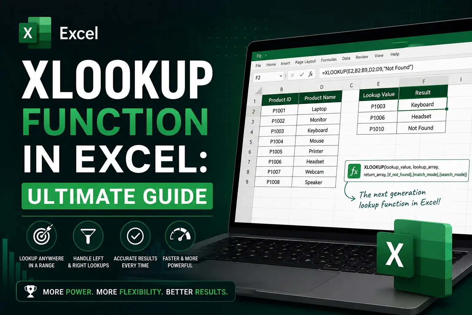
XLOOKUP is Excel’s modern, flexible lookup function. It replaces many common uses of VLOOKUP, HLOOKUP, and INDEX/MATCH. XLOOKUP is available in Microsoft 365, Excel 2021, Excel 2024, and Excel for the web.

---

XLOOKUP Syntax

=XLOOKUP(lookup_value, lookup_array, return_array, [if_not_found], [match_mode], [search_mode])

Argument	Required?	Description
lookup_value	Yes	The value you want to find.
lookup_array	Yes	The range or array to search.
return_array	Yes	The range or array containing the value to return.
if_not_found	Optional	Value to return if no match is found. If omitted, XLOOKUP returns #N/A.
match_mode	Optional	Controls exact, approximate, or wildcard matching.
search_mode	Optional	Controls search direction and method.

---

XLOOKUP Match Modes

match_mode	Meaning
0	Exact match. This is the default.
-1	Exact match. If not found, return the next smaller item.
1	Exact match. If not found, return the next larger item.
2	Wildcard match. Supports *, ?, and ~.

Examples:

=XLOOKUP(A2, B2:B100, C2:C100)

Uses exact match because 0 is the default.

=XLOOKUP(A2, B2:B100, C2:C100, "Not Found", 0)

Explicit exact match.

=XLOOKUP(A2, B2:B100, C2:C100, "Not Found", -1)

Exact match, or next smaller value if not found.

=XLOOKUP(A2, B2:B100, C2:C100, "Not Found", 1)

Exact match, or next larger value if not found.

=XLOOKUP("*" & A2 & "*", B2:B100, C2:C100, "Not Found", 2)

Wildcard match.

---

XLOOKUP Search Modes

search_mode	Meaning
1	Search first-to-last. This is the default.
-1	Search last-to-first. Useful for finding the last match.
2	Binary search. Lookup array should be sorted ascending.
-2	Binary search. Lookup array should be sorted descending.

Example:

=XLOOKUP(A2, B2:B100, C2:C100, "Not Found", 0, -1)

This searches from bottom to top and returns the last match.

---

Basic XLOOKUP Example

Assume this table:

	A	B	C	D
1	ID	Product	Price	Stock
2	101	Pen	2.50	100
3	102	Notebook	4.00	50
4	103	Eraser	1.25	200

Basic formula:

=XLOOKUP(102, A2:A4, C2:C4)

Result:

4.00

Explanation:

• Look for 102
• Search in A2:A4
• Return the matching value from C2:C4
• Use exact match by default

Return a Different Column

=XLOOKUP(102, A2:A4, B2:B4)

Result:

Notebook

Use a Cell Reference

If cell F1 contains 102:

=XLOOKUP(F1, A2:A4, C2:C4)

Result:

4.00

Return a Message If Not Found

=XLOOKUP(F1, A2:A4, C2:C4, "Product not found")

If the ID does not exist, Excel returns:

Product not found

---

XLOOKUP Uses Exact Match by Default

Unlike VLOOKUP, XLOOKUP does not require you to specify exact match in most cases.

These are equivalent:

=XLOOKUP(A2, B2:B100, C2:C100)

=XLOOKUP(A2, B2:B100, C2:C100, , 0)

=XLOOKUP(A2, B2:B100, C2:C100, "Not Found", 0)

For teaching or documentation purposes, you may explicitly include 0, but it is not required.

---

XLOOKUP Can Look Left

One of XLOOKUP’s biggest advantages is that it can look to the left.

Assume:

	A	B	C
1	Product	ID	Price
2	Pen	101	2.50
3	Notebook	102	4.00
4	Eraser	103	1.25

You want to find the product name using the ID in column B.

Formula:

=XLOOKUP(102, B2:B4, A2:A4)

Result:

Notebook

VLOOKUP cannot do this directly because VLOOKUP only searches the first column of the lookup range.

---

XLOOKUP vs VLOOKUP

VLOOKUP version

=VLOOKUP(102, A2:D4, 3, FALSE)

XLOOKUP version

=XLOOKUP(102, A2:A4, C2:C4, "Not Found")

XLOOKUP is often easier because:

• No column number is needed
• Exact match is the default
• It can look left
• It has built-in error handling
• It can return multiple columns
• It works vertically and horizontally

Common Conversion

VLOOKUP:

=VLOOKUP(A2, A2:D100, 3, FALSE)

XLOOKUP:

=XLOOKUP(A2, A2:A100, C2:C100, "Not Found")

---

XLOOKUP vs HLOOKUP

Assume this horizontal table:

	B	C	D
1	Jan	Feb	Mar
2	500	600	700

HLOOKUP version:

=HLOOKUP("Feb", B1:D2, 2, FALSE)

XLOOKUP version:

=XLOOKUP("Feb", B1:D1, B2:D2, "Not Found")

Result:

600

---

XLOOKUP vs INDEX/MATCH

INDEX/MATCH version:

=INDEX(C2:C100, MATCH(A2, B2:B100, 0))

XLOOKUP version:

=XLOOKUP(A2, B2:B100, C2:C100, "Not Found")

Use INDEX/MATCH when you need compatibility with older Excel versions.

Use XLOOKUP when you have Microsoft 365, Excel 2021, or newer.

---

XLOOKUP from Another Sheet

If the lookup data is on another sheet:

=XLOOKUP(A2, Sheet2!A2:A100, Sheet2!C2:C100, "Not Found")

If the sheet name contains spaces:

=XLOOKUP(A2, 'Price List'!A2:A100, 'Price List'!C2:C100, "Not Found")

If the workbook is external:

=XLOOKUP(A2, '[PriceList.xlsx]Sheet1'!$A$2:$A$100, '[PriceList.xlsx]Sheet1'!$C$2:$C$100, "Not Found")

---

XLOOKUP with Excel Tables

XLOOKUP works very well with Excel Tables.

Assume a table named Products with columns:

• ID
• Product
• Price
• Stock

Formula:

=XLOOKUP(A2, Products[ID], Products[Price], "Not Found")

If the formula is inside the same table, you may use structured references like:

=XLOOKUP([@ID], Products[ID], Products[Price], "Not Found")

Benefits of using tables:

• Ranges expand automatically
• Formulas are easier to read
• Column names reduce mistakes
• No need to lock ranges with $

---

XLOOKUP with Named Ranges

If you define named ranges:

• ProductIDs
• ProductPrices

Then:

=XLOOKUP(A2, ProductIDs, ProductPrices, "Not Found")

This can make formulas more readable.

---

Return Multiple Columns with XLOOKUP

In Microsoft 365 and newer Excel versions, XLOOKUP can return multiple columns at once.

Assume:

	A	B	C	D
1	ID	Product	Price	Stock
2	101	Pen	2.50	100
3	102	Notebook	4.00	50
4	103	Eraser	1.25	200

Formula:

=XLOOKUP(102, A2:A4, B2:D4, "Not Found")

Result spills into neighboring cells:

Notebook    4.00    50

This replaces several separate formulas:

=XLOOKUP(102, A2:A4, B2:B4)
=XLOOKUP(102, A2:A4, C2:C4)
=XLOOKUP(102, A2:A4, D2:D4)

---

Lookup Multiple Values at Once

If F2:F4 contains multiple lookup IDs:

=XLOOKUP(F2:F4, A2:A100, B2:B100, "Not Found")

Excel can return multiple results as a spilled array.

Example:

If F2:F4 contains:

101
102
103

The formula can return:

Pen
Notebook
Eraser

---

Horizontal Lookup with XLOOKUP

XLOOKUP can replace HLOOKUP.

Assume:

	A	B	C	D
1	Metric	Jan	Feb	Mar
2	Sales	500	600	700
3	Costs	300	350	400
4	Profit	200	250	300

Return February sales:

=XLOOKUP("Feb", B1:D1, B2:D2)

Result:

600

Return all February values:

=XLOOKUP("Feb", B1:D1, B2:D4)

Result:

600
350
250

---

Two-Way Lookup with XLOOKUP

You can nest XLOOKUP to lookup by both row and column.

Assume:

	A	B	C	D
1	Metric	Jan	Feb	Mar
2	Sales	500	600	700
3	Costs	300	350	400
4	Profit	200	250	300

Inputs:

• F1 = Month
• G1 = Metric

Formula:

=IFNA(XLOOKUP($F$1, $B$1:$D$1, XLOOKUP($G$1, $A$2:$A$4, $B$2:$D$4)), "Not Found")

Example:

• F1 = Feb
• G1 = Sales

Result:

600

How it works:

1. The inner XLOOKUP finds the correct row based on the metric.
2. The outer XLOOKUP finds the correct column based on the month.
3. The intersection value is returned.

---

Approximate Match with XLOOKUP

XLOOKUP can perform approximate lookups using match_mode.

Next Smaller Match: -1

Useful for:

• Tax brackets
• Commission tiers
• Discount levels
• Grade boundaries

Example:

	F	G
1	Sales	Commission
2	0	0%
3	1000	5%
4	5000	10%
5	10000	15%

Formula:

=XLOOKUP(7000, F2:F5, G2:G5, "Not Found", -1)

Result:

10%

Why?

• 7000 is between 5000 and 10000.
• XLOOKUP returns the next smaller threshold: 5000.
• The corresponding commission is 10%.

For bracket-style tables, it is usually best to sort the lookup values.

Next Larger Match: 1

Use this when you need the next higher threshold.

=XLOOKUP(7000, F2:F5, G2:G5, "Not Found", 1)

This can be useful for:

• Shipping weight bands
• Minimum order tiers
• Price ranges
• Service level thresholds

For predictable results, keep the lookup values sorted consistently.

---

Wildcard Match with XLOOKUP

Use match_mode = 2 for wildcard matching.

Wildcard	Meaning
*	Matches any number of characters
?	Matches one character
~	Escapes a wildcard character

---

Partial Text Lookup

If cell F1 contains:

note

Formula:

=XLOOKUP("*" & F1 & "*", A2:A100, B2:B100, "Not Found", 2)

This searches for any value containing:

note

It can match:

Notebook
Note Pad
Sticky Notes

Important:

Wildcards are treated specially only when match_mode is 2.

Search for Literal Wildcards

To search for an actual asterisk:

=XLOOKUP("~*", A2:A100, B2:B100, "Not Found", 2)

To search for an actual question mark:

=XLOOKUP("~?", A2:A100, B2:B100, "Not Found", 2)

To search for an actual tilde:

=XLOOKUP("~~", A2:A100, B2:B100, "Not Found", 2)

---

Find the First or Last Match

By default, XLOOKUP searches from first to last.

Assume:

	A	B
1	ID	Value
2	101	First
3	101	Second
4	101	Third

Default formula:

=XLOOKUP(101, A2:A4, B2:B4)

Returns:

First

To return the last match:

=XLOOKUP(101, A2:A4, B2:B4, "Not Found", 0, -1)

Returns:

Third

---

Binary Search Mode for Large Sorted Data

If your lookup column is sorted, you can use binary search for better performance.

Ascending binary search

=XLOOKUP(A2, B2:B100000, C2:C100000, "Not Found", 0, 2)

Use this when B2:B100000 is sorted ascending.

Descending binary search

=XLOOKUP(A2, B2:B100000, C2:C100000, "Not Found", 0, -2)

Use this when B2:B100000 is sorted descending.

Important:

Binary search modes require the lookup array to be sorted correctly. If the data is not sorted properly, results may be incorrect.

---

XLOOKUP with Multiple Criteria

XLOOKUP does not have a built-in “multiple criteria” argument, but there are several reliable ways to handle multiple conditions.

Method 1: Helper Key Column

This is often the simplest and fastest method.

Assume:

	A	B	C	D
1	Region	Product	Sales	Key
2	East	Pen	100	East
3	West	Pen	120	West
4	East	Ruler	80	East

Helper formula in column D:

=A2 & "|" & B2

Lookup formula:

=XLOOKUP(F1 & "|" & G1, D2:D100, C2:C100, "Not Found")

Where:

• F1 contains Region
• G1 contains Product
• Column D contains the helper key
• Column C contains the return value

Method 2: Concatenate Arrays Directly

In Microsoft 365, you can combine ranges directly:

=XLOOKUP(F1 & "|" & G1, A2:A100 & "|" & B2:B100, C2:C100, "Not Found")

This avoids a helper column but may be slower on very large ranges.

Method 3: Boolean Array Lookup

=XLOOKUP(1, (A2:A100=F1) * (B2:B100=G1), C2:C100, "Not Found")

This searches for rows where both conditions are true.

Example:

• F1 = East
• G1 = Pen

The formula returns the matching sales value.

If You Need All Matches, Use FILTER

XLOOKUP returns only one match.

To return all matches:

=FILTER(C2:C100, (A2:A100=F1) * (B2:B100=G1), "No matches")

---

XLOOKUP and Dynamic Arrays

XLOOKUP is designed to work with dynamic arrays.

Returning multiple columns

=XLOOKUP(A2, B2:B100, C2:E100, "Not Found")

Looking up multiple values

=XLOOKUP(A2:A10, B2:B100, C2:C100, "Not Found")

Returning arrays from formulas

=XLOOKUP(A2, B2:B100, C2:E100, "Not Found")

If the result needs multiple cells, Excel spills the result into adjacent cells.

---

Error Handling in XLOOKUP

Use the built-in if_not_found argument

=XLOOKUP(A2, B2:B100, C2:C100, "Not Found")

This is usually the best approach.

Return blank instead of #N/A

=XLOOKUP(A2, B2:B100, C2:C100, "")

Use IFNA

=IFNA(XLOOKUP(A2, B2:B100, C2:C100), "Not Found")

Use IFERROR

=IFERROR(XLOOKUP(A2, B2:B100, C2:C100), "Error")

Use IFERROR carefully because it can hide real formula problems.

---

Common XLOOKUP Errors

#N/A

Meaning

No match was found, and no if_not_found value was provided.

Fix

=XLOOKUP(A2, B2:B100, C2:C100, "Not Found")

#VALUE!

Common Causes

• lookup_array and return_array are different sizes
• Invalid match mode
• Invalid search mode
• Incorrect range syntax

Fix

Make sure the ranges align.

Wrong:

=XLOOKUP(A2, B2:B100, C2:C90)

Correct:

=XLOOKUP(A2, B2:B100, C2:C100)

#NAME?

Meaning

Excel does not recognize the function.

Common Cause

You are using an older version of Excel that does not support XLOOKUP.

Fix

Use INDEX/MATCH:

=INDEX(C2:C100, MATCH(A2, B2:B100, 0))

#SPILL!

Meaning

XLOOKUP is returning multiple values, but the spill range is blocked.

Fix

Clear the cells where the result needs to spill.

---

Troubleshooting Wrong Results

Problem 1: Numbers stored as text

If the lookup value is numeric but the lookup column contains text, XLOOKUP may not find a match.

Example:

Lookup value:

102

Lookup column contains:

"102"

Possible fixes:

Convert the lookup column to numbers.

Or convert the lookup value to text:

=XLOOKUP(TEXT(A2, "0"), B2:B100, C2:C100, "Not Found")

Or convert the lookup value to a number:

=XLOOKUP(VALUE(A2), B2:B100, C2:C100, "Not Found")

Problem 2: Extra spaces

Extra spaces can prevent matches.

Use TRIM:

=XLOOKUP(TRIM(A2), B2:B100, C2:C100, "Not Found")

If the source data contains spaces, clean the source data too.

Problem 3: Dates stored as text

XLOOKUP works best with real Excel dates.

Use:

=XLOOKUP(DATE(2025,2,1), A2:A100, B2:B100, "Not Found")

If your dates are text, convert them to real dates first.

Problem 4: Duplicate lookup values

XLOOKUP returns only one match.

Use default search mode for the first match:

=XLOOKUP(A2, B2:B100, C2:C100, "Not Found")

Use search mode -1 for the last match:

=XLOOKUP(A2, B2:B100, C2:C100, "Not Found", 0, -1)

Use FILTER for all matches:

=FILTER(C2:C100, B2:B100=A2, "No matches")

Problem 5: Case sensitivity

XLOOKUP is not case-sensitive.

These are treated as the same:

ABC
abc
AbC

For case-sensitive lookup, use FILTER with EXACT:

=FILTER(C2:C100, EXACT(A2:A100, F1), "Not Found")

Or use INDEX/MATCH with EXACT:

=INDEX(C2:C100, MATCH(TRUE, EXACT(A2:A100, F1), 0))

In older environments, the INDEX/MATCH version may require Ctrl + Shift + Enter.

---

XLOOKUP with Dates

Exact date lookup

=XLOOKUP(DATE(2025,2,1), A2:A100, B2:B100, "Not Found")

Approximate date lookup

Assume:

	F	G
1	Start Date	Rate
2	2025-01-01	Low
3	2025-02-01	Medium
4	2025-03-01	High

Formula:

=XLOOKUP(DATE(2025,2,15), F2:F4, G2:G4, "Not Found", -1)

Result:

Medium

For date bracket tables, sort the dates appropriately.

---

XLOOKUP Limitations

Not available in older Excel versions

XLOOKUP is not available in:

• Excel 2019
• Excel 2016
• Excel 2013
• Excel 2010

For compatibility, use INDEX/MATCH or VLOOKUP.

Not case-sensitive

XLOOKUP cannot directly distinguish between:

ABC
abc

Use EXACT with FILTER or INDEX/MATCH for case-sensitive lookups.

Returns only one match

XLOOKUP returns the first or last match depending on search mode.

Use FILTER if you need all matches.

Approximate match requires care

For approximate match modes, sorted data gives more predictable results.

For binary search modes, sorted data is required.

---

Frequently Asked Questions

Is XLOOKUP better than VLOOKUP?

Usually, yes. XLOOKUP is more flexible, easier to read, and does not require column index numbers.

Is XLOOKUP exact by default?

Yes. XLOOKUP uses exact match by default.

Can XLOOKUP look left?

Yes.

Example:

=XLOOKUP(A2, C2:C100, A2:A100)

Can XLOOKUP return multiple values?

Yes. In Microsoft 365 and newer Excel versions, XLOOKUP can return multiple columns or multiple rows as a spilled array.

Can XLOOKUP return all matches?

Not directly. XLOOKUP returns one match. Use FILTER to return all matches.

Is XLOOKUP case-sensitive?

No. XLOOKUP is not case-sensitive.

For case-sensitive lookup, use EXACT with FILTER or INDEX/MATCH.

Does XLOOKUP work with wildcards?

Yes, but only when match_mode is 2.

=XLOOKUP("*" & A2 & "*", B2:B100, C2:C100, "Not Found", 2)

Does XLOOKUP require sorted data?

Exact match does not require sorted data.

Approximate match modes work best with sorted data, and binary search modes require sorted data.

Why does XLOOKUP return #NAME?

Your Excel version may not support XLOOKUP. Use Microsoft 365, Excel 2021, Excel 2024, or Excel for the web.

Why does XLOOKUP return #SPILL?

The formula is returning multiple values, but something is blocking the spill range.

Clear the cells where the result needs to spill.

Can XLOOKUP replace HLOOKUP?

Yes.

HLOOKUP:

=HLOOKUP("Feb", B1:D3, 2, FALSE)

XLOOKUP:

=XLOOKUP("Feb", B1:D1, B2:D2, "Not Found")

Can XLOOKUP replace INDEX/MATCH?

Yes, in most common cases.

INDEX/MATCH:

=INDEX(C2:C100, MATCH(A2, B2:B100, 0))

XLOOKUP:

=XLOOKUP(A2, B2:B100, C2:C100, "Not Found")

---

Final Summary

XLOOKUP is the most flexible built-in lookup function in modern Excel.

A good default formula is:

=XLOOKUP(lookup_value, lookup_array, return_array, "Not Found")

Use XLOOKUP when you need:

• Exact lookup
• Left lookup
• Right lookup
• Horizontal lookup
• Multi-column return
• Built-in error handling
• Last-match lookup
• Approximate match
• Wildcard match
• Dynamic array results